
Advanced Features
Contents
Advanced Features#
This page covers advanced NeurEco Tabular features for model analysis and optimization.
On this page
Sensitivity Analysis#
Sensitivity analysis helps you understand which input features have the most impact on model outputs. This functionality is based on input perturbation: NeurEco adds perturbations of different magnitudes to each node, calculates the corresponding variation of the output, and deduces the importance ranking of nodes.
This can reveal:
Which inputs are truly important
Which inputs could be removed without losing accuracy
Potential issues with data or model
If an input feature has little impact on the outputs, it can be excluded from training. The new training with fewer input features generally leads to a smaller model without significant loss of accuracy.
Single Sample Analysis#
1. Switch to the Evaluation panel
2. Choose the file in Evaluation files section:
If the file was supplied earlier, it is already listed
To add a new file, press + in the Additional section
For sensitivity analysis, the output file is not required
3. Select a sample using the Sample slider
4. Click on one of the output neurons on the network plot in the Network sensitivity section
Each neuron becomes colored according to its sensitivity
Click on an input neuron to see its calculated sensitivity value
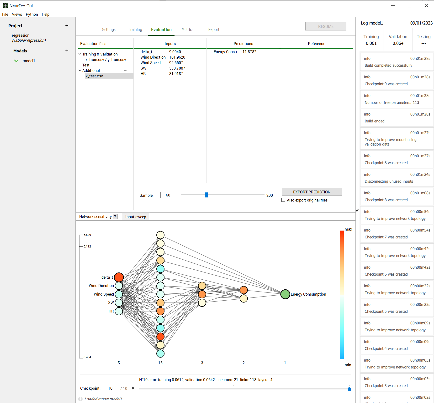
Network sensitivity for a single sample#
Use gradient computation for sensitivity analysis:
import numpy as np

# Get model weights
w = model.get_weights()
x = x_test[0:1]  # Single sample

# Compute gradient of each output w.r.t. inputs
n_outputs = model.get_output_count()

for out_idx in range(n_outputs):
    py = np.zeros((1, n_outputs))
    py[0, out_idx] = 1.0  # Unit perturbation for this output

    pw, px = model.gradient(w, x, py)

    print(f"Output {out_idx} sensitivity to inputs: {px.flatten()}")
Dataset-Wide Analysis#
The sensitivity for a whole dataset is calculated as a norm of sensitivities on each sample.
1. Switch to the Metrics panel
2. Choose the file in Evaluation files section
3. Click on one of the output neurons on the network plot
Each neuron becomes colored according to its aggregated sensitivity
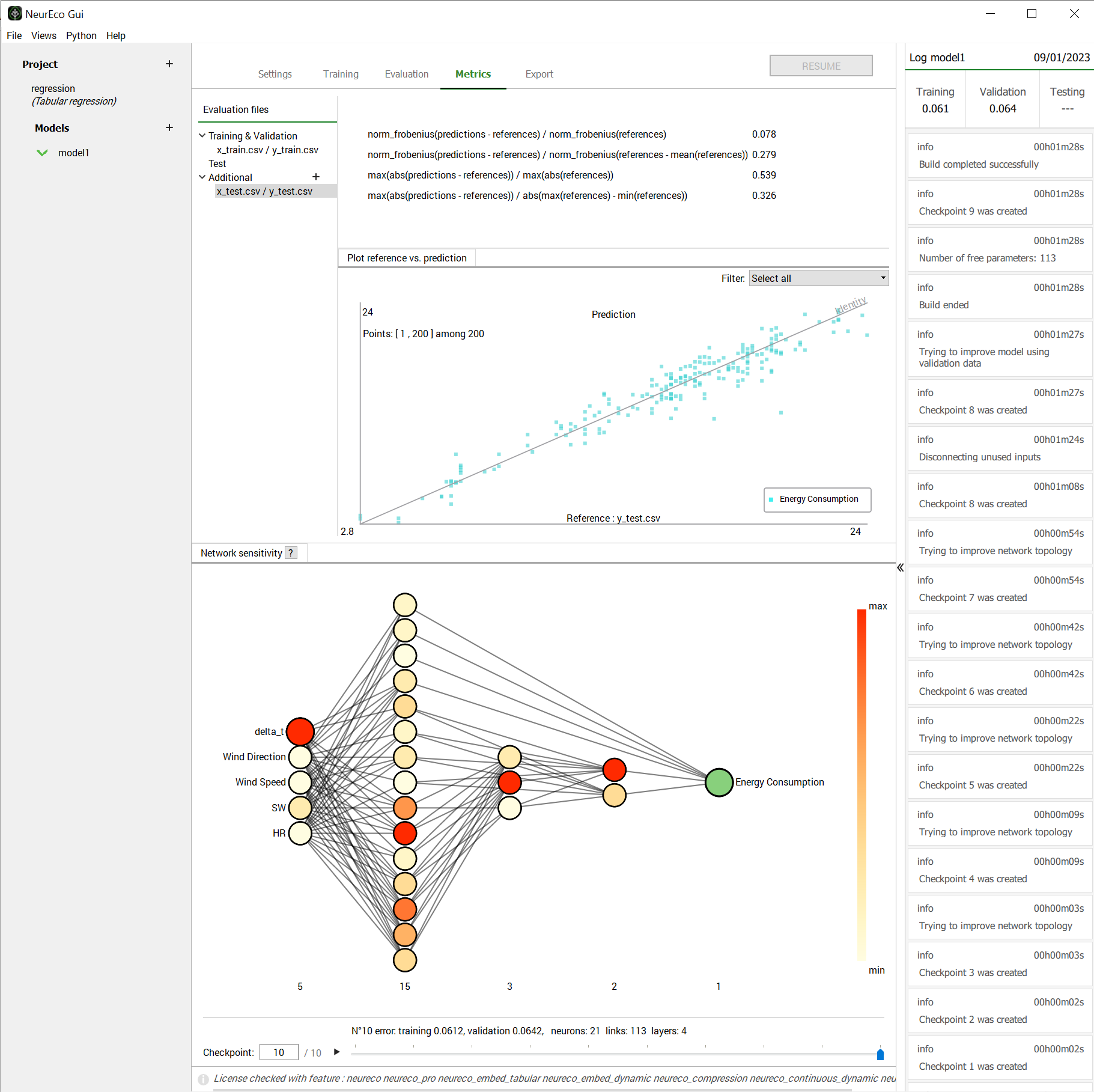
Network sensitivity aggregated over a dataset#
import numpy as np

w = model.get_weights()
n_outputs = model.get_output_count()
n_inputs = model.get_input_count()

# Aggregate sensitivities over all samples
sensitivities = np.zeros((n_outputs, n_inputs))

for out_idx in range(n_outputs):
    py = np.zeros((len(x_test), n_outputs))
    py[:, out_idx] = 1.0

    pw, px = model.gradient(w, x_test, py)

    # Norm over samples
    sensitivities[out_idx] = np.linalg.norm(px, axis=0)

print("Sensitivity matrix (outputs x inputs):")
print(sensitivities)
Note
By default, network sensitivity is performed with the last model available in the checkpoint. Use the checkpoint slider to choose any other available model.
Input Sweep#
Input sweep analysis shows how the model’s output responds to changes in a single input variable while holding all other inputs constant. This is useful for:
Sensitivity analysis: Understanding which inputs have the greatest effect
Model interpretation: Visualizing learned input-output relationships
Validation: Checking that the model behaves as expected across the input range
Warning
Sweeping one input while the others stay fixed can leave the domain covered by the training data, especially when the inputs are correlated. In such regions the model extrapolates, and its predictions should be treated with caution — an implausible-looking sweep far from the sample point does not necessarily mean the model is bad. The GUI shows this disclaimer under the Input sweep legend.
1. Switch to the Evaluation panel
2. Click on Input sweep
3. Choose a dataset from Evaluation files and click on it
4. Choose a sample using the Sample slider
5. In the Input sweep window, set the Input and Outputs
Multiple output features can be plotted in the same graph
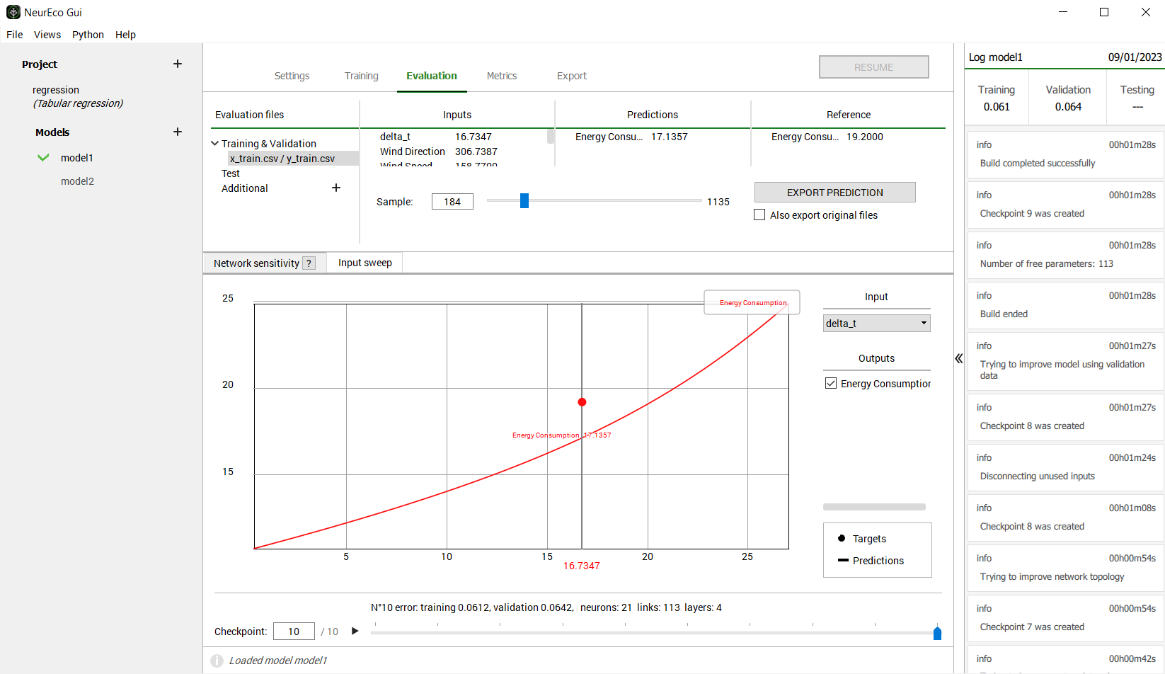
Input sweep showing output response as one input varies#
Use the perform_input_sweep method:
import numpy as np

# Define a sample input (e.g., model has 5 inputs)
sample = np.array([1.0, 2.5, 0.5, 3.0, 1.5])

# Sweep input 0 from -5 to 5, observing output 0
model.perform_input_sweep(
    input_feature=sample,
    input_id=0,
    input_interval=[-5, 5],
    output_id=0
)
Save without displaying:
model.perform_input_sweep(
    input_feature=sample,
    input_id=0,
    input_interval=[-5, 5],
    output_id=0,
    show=False,
    save_path="input_sweep_analysis.png"
)
Higher resolution sweep:
model.perform_input_sweep(
    input_feature=sample,
    input_id=0,
    input_interval=[-5, 5],
    output_id=0,
    n_points=500
)
Analyze all inputs:
n_inputs = model.get_input_count()
sample = np.random.randn(n_inputs)

for i in range(n_inputs):
    model.perform_input_sweep(
        input_feature=sample,
        input_id=i,
        input_interval=[-3, 3],
        output_id=0,
        show=False,
        save_path=f"sweep_input_{i}.png"
    )
    print(f"Saved sweep for input {i}")
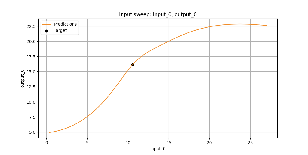
Input sweep analysis with marker showing the initial sample point#
Method Reference#
model.perform_input_sweep(
    input_feature,      # 1-D array: sample values (held constant except swept input)
    input_id,           # Index of input to sweep (0-based)
    input_interval,     # [min, max] range for the sweep
    output_id,          # Index of output to plot (0-based)
    n_points=100,       # Number of evaluation points
    show=True,          # Display plot interactively
    save_path=None      # Path to save figure (optional)
)
Interpreting the Plot#
The input sweep plot shows:
X-axis: The swept input variable across the specified interval
Y-axis: The model’s predicted output value
Curve: How the output changes as the input varies
Marker: The output value at the original sample point
Key observations:
Steep slopes indicate high sensitivity to that input
Curves indicate nonlinear relationships learned by the model
Flat regions indicate the input has little effect in that range
Gradient Computation#
NeurEco provides automatic differentiation for integration with optimization algorithms and advanced analysis.
Overview#
A NeurEco Tabular model can be represented as a function:
where \(x\) is the input, \(w\) are the model weights, and \(y\) is the output.
NeurEco provides two modes of automatic differentiation:
Forward mode (tangent mode): Computes how output perturbations result from input and weight perturbations
Backward mode (adjoint mode): Computes gradients with respect to weights and inputs given output perturbations
This allows NeurEco models to be used as differentiable blocks within optimization problems, neural network training loops, or any workflow requiring gradient information.
Note
Gradient and derivative computation is only available for the Tabular solution in the Python API.
Available Methods#
Method |
Description |
|---|---|
|
Retrieve the model’s current weights |
|
Set the model’s weights to user-defined values |
|
Compute forward mode automatic differentiation (tangent mode) |
|
Compute backward mode automatic differentiation (adjoint mode) |
get_weights / set_weights#
# Get current weights
weights = model.get_weights()
print(f"Model has {len(weights)} parameters")

# Modify weights (e.g., add small perturbation)
weights_modified = weights + 0.01 * np.random.randn(*weights.shape)

# Set the new weights
status = model.set_weights(weights_modified)
forward_derivative#
Compute how perturbations in weights (\(dw\)) and inputs (\(dx\)) propagate to output perturbations (\(dy\)):
import numpy as np

# Get model weights
w = model.get_weights()

# Define input data
x = np.random.randn(100, 5)  # 100 samples, 5 inputs

# Define perturbations
dw = np.random.randn(*w.shape) * 0.01  # Small weight perturbation
dx = np.random.randn(*x.shape) * 0.01  # Small input perturbation

# Compute forward derivative
dy = model.forward_derivative(w, dw, x, dx)
print(f"Output perturbation shape: {dy.shape}")
gradient#
Compute gradients with respect to weights and inputs given an output perturbation \(py\):
import numpy as np

# Get model weights
w = model.get_weights()

# Define input data
x = np.random.randn(100, 5)  # 100 samples, 5 inputs

# Define output perturbation (e.g., gradient of a loss function)
py = np.ones((100, 2))  # 100 samples, 2 outputs

# Compute gradients
pw, px = model.gradient(w, x, py)

print(f"Weight gradient shape: {pw.shape}")
print(f"Input gradient shape: {px.shape}")
Use Case: Optimization with NeurEco#
Use the NeurEco model as a differentiable block within an optimization problem:
import numpy as np
from scipy.optimize import minimize

def objective(x):
    """Objective function using NeurEco model."""
    y = model.evaluate(x.reshape(1, -1))
    return np.sum(y**2)  # Example: minimize sum of squared outputs

def objective_gradient(x):
    """Gradient of objective function."""
    w = model.get_weights()
    x_2d = x.reshape(1, -1)
    y = model.evaluate(x_2d)

    # Gradient of sum(y^2) w.r.t. y is 2*y
    py = 2 * y

    # Get gradient w.r.t. inputs
    pw, px = model.gradient(w, x_2d, py)

    return px.flatten()

x0 = np.random.randn(5)
result = minimize(objective, x0, jac=objective_gradient, method='BFGS')
print(f"Optimal input: {result.x}")
Network Visualization#
Visualize the structure of your NeurEco neural network.
The network structure is displayed in the main interface showing:
Network architecture
Layer structure
Connection patterns
Neuron activations (during sensitivity analysis)
# Plot the network structure
model.plot_network()

# Save to file
model.plot_network(save_to="network_structure.png")
The visualization shows how NeurEco’s parsimonious architecture differs from traditional layered networks — neurons can connect to any other neuron, not just adjacent layers.
Compression Coefficient Analysis#
For Compression models, you can analyze the relationships between compression coefficients to discover patterns in your data.
In the Compression Coefficients panel:
View 2D or 3D plots of coefficient relationships
Use the closed-shape selection tool to identify clusters
Export selected data groups
Discover hidden patterns or classes in your data
The Compressor model provides a built-in method to visualize the latent space:
Basic 2D plot:
# Plot compression coefficients (first 2 dimensions by default)
model.plot_compression_coefficients(
    data_to_compress=x_train,
    title="Compression Coefficient Space"
)
3D plot with specific dimensions:
# Plot 3 specific latent dimensions
model.plot_compression_coefficients(
    data_to_compress=x_train,
    neurons_ids=[0, 1, 2],  # First 3 dimensions
    title="3D Latent Space"
)
With categorical labels:
# Color points by category (e.g., data source or class)
labels = ["Type A"] * 50 + ["Type B"] * 50  # Example labels
model.plot_compression_coefficients(
    data_to_compress=x_train,
    data_labels=labels,
    title="Latent Space by Category"
)
With continuous colormap:
# Color points by a continuous value (e.g., time index)
values = np.arange(len(x_train))  # Example: sample index
model.plot_compression_coefficients(
    data_to_compress=x_train,
    data_labels=values,
    title="Latent Space by Sample Index",
    save_path="latent_space.png"
)
Use cases:
Discover natural clustering in your data
Identify anomalies (points far from clusters)
Understand data structure in reduced dimensions
Model Size Control#
Control the size of your NeurEco network during training.
Links Maximum Number#
Limit the total number of connections in the network:
config = Tabular.RegressorBuildConfig(
    input_data=x_train,
    output_data=y_train,
    write_model_to="model.ednn",
    links_maximum_number=100,  # Maximum 100 connections
)
Use this when:
Deploying to memory-constrained devices
Needing faster inference
Preferring simpler, more interpretable models
Disconnect Unused Inputs#
NeurEco can automatically disconnect inputs that don’t contribute to predictions. Each time it changes the network structure, it may prune the links from the inputs, and with final_learning=True the final steps include a pass that disconnects the remaining unused inputs. With disconnect_inputs_if_possible=False, NeurEco never prunes a link from an input and can also prune fewer of the other links, so expect a larger network. The setting is on by default:
config = Tabular.RegressorBuildConfig(
    # ...
    disconnect_inputs_if_possible=True,  # Default: True
)
After training, check which inputs are still connected:
# The model may have fewer effective inputs than provided
# Use sensitivity analysis to see which inputs are used
Resume Training#
Continue training from a checkpoint with modified settings:
config = Tabular.RegressorBuildConfig(
    input_data=x_train,
    output_data=y_train,
    write_model_to="model_v2.ednn",
    checkpoint_to_start_build_from="./model/model.checkpoint",
    start_build_from_model_number=5,  # Model index 5 of the checkpoint (-1 = last)
    freeze_structure=False,  # Allow architecture changes
)

model.build(config)
Options:
freeze_structure=True: Keep architecture, retrain weights (requiresfinal_learning=True)freeze_structure=False: Allow continued architecture enrichment